Project: Can collector
Data: Fall 2020
Yanda Cheng(yc2675)
Jinling Sun(js 3567)
Final Demo Video
Objective
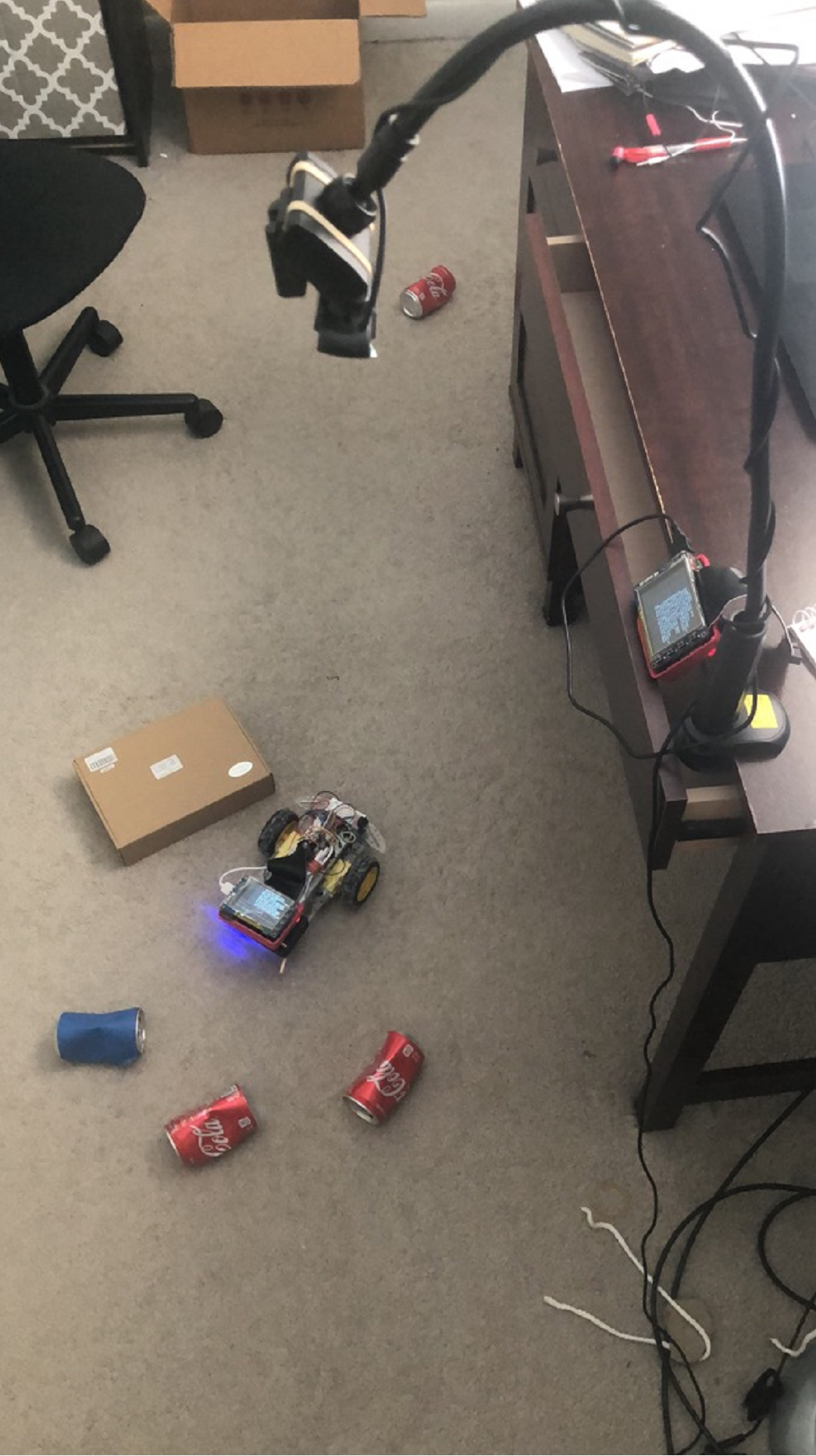
Our project aim to design a fully automated robot which is able to collect the target object during the job routine. The robot shall classify the cans as beer cans and cola cans lying on the ground. our robot will run on the ground and detect cans. If a can is detected, the robot will recognize the can and push forward the can to the designated place according to its category. After classification, our algorithm will implement the segmentation algorithm which labels all pixels that belong to the can. With the can segmentation output image, we can compute the angle for the robot to push the cans . Finally, we will design a way to push the can to its destination. We have a camera collecting pictures by vision system RPI and sending moving commands to robot RPi. After analyzing these images, the vision system RPi RPI controls the motors of car RPI to move the robot and displays the result on the PiTFT. The figure below shows the basic overview of our project (top), Car Robot (bot, left) Vision system(bot,righ)
Introduction
For this project, we designed two systems which are the motor control system and the camera vision system. In the camera vision system, the robot can correctly segment the ground from the rest of the image so that our vehicle will not run into the walls or chairs and while roaming on the floor, the RPI of vision system will detect the cans and classify the cans to different categories. The final result of the vision system from the image will be delivered to the PID control program, and the motor control program will calculate the best pathway for the robot to collect the can on the ground and return to the final destination. The data transfer through the socket through wifi will only be a simple command for motor control. As the final result, our robot will keep collecting cans on the ground and stay on the final position waiting for any new target object to occur in the vision system. Once we turn on the system, the robot could work the entire day with the full charge. The RPI low cost and low power consumption advantages make this robot have potential to be marketed as a trash collector in future.
Design
Software tools and packages
In our project, there was a vehicle on the floor that could move around and push the cans to designated destinations. There was a camera on top of the floor that could ‘see’ the vehicle, cans and obstacles on the ground. Two Raspberry Pis were used in our project. One was connected to the camera, it gathered images from the camera, analyzed them and then sent commands to another Pi, which was responsible for the movements of the vehicle.
Software tools
Tensorflow
Tensorflow is a deep learning package that provides a collection of workflows to develop, train, and deploy models using Python. It’s one of the most widely used tools in the deep learning area.
Tensorflow-lite
Tensorflow-lite also referred to as tf-lite, is the tool that can convert the models trained by TensorFlow (in .hdf5 format in our project) to a file in .tflite format, which can be used in the embedded system platforms such as Raspberry Pi. For how to install tensorflow-lite, please refer to:
https://qengineering.eu/install-tensorflow-2-lite-on-raspberry-pi-4.html
To convert the tensorflow model into tf-lite model, activate the environment with tensorfow of vesion above 2.0, run the following model:tflite_convert --keras_model_file=model.hdf5 --output_file=model.tfliteWhere model.hdf is the model name, and model.tflite is the generated model name.
Opencv
Opencv is an image processing tool which includes many useful methods and algorithms. In our project, we used it for some basic image processing, such as resizing and permuting axes of an array.
Socket
A network socket is a software structure within a network node of a computer network that serves as an endpoint for sending and receiving data across the network. In our project, the socket is used for sending commands from the camera Pi, which is responsible for computer vision and control algorithms, to the vehicle Pi, which is responsible for moving the vehicle.
Computer Vision
Deep Learning ModelIn our computer vision algorithm, the deep learning model fulfilled three tasks, object detection, segmentation and classification. The object detection task helped us find all objects, no matter what categories they belong to. It is the fundamental part of the computer vision algorithm because further analysis must be done after all objects have been found. The object classification is a crucial part of our algorithm. To fulfil our tasks, we should know which objects are cola cans and which are beer cans, which object is our vehicle and then control the vehicle to push different cans to their designated destinations. Any error in the classification will lead to wrong movement of the vehicle. Or, if the cans were misclassified, they will be pushed to wrong destinations. Object segmentation is the basis for further analysis. Many of the traditional image analysis are based on the segmentation results. For example, we should use the segmentation results of the cans to precisely compute the positions of the cans. Vehicle segmentation results are necessary for computing the direction, angle and position of the vehicle. The algorithms that do not involve deep learning methods are referred to as traditional algorithms in our project. These algorithms act as the mediate between the computer vision algorithms and the control algorithms. The traditional algorithms compute the positions of objects, the direction and position of vehicles and work out a route for the vehicle to circumvent the obstacles and push the cans to designated destinations.
Deep Learning Model Development
As mentioned above, our project involves object detection, segmentation, and classification. A good candidate deep learning model for fulfilling these requirements seems to be Mask-RCNN. Mask-RCNN first uses a ConvNet to extract feature maps from the images, then the features maps are passed through a Region Proposal Network (RPN) to generate candidate bounding boxes, then ROI pooling layer resizes all the candidate bounding boxes to the same size and recognize the objects in these bounding boxes, finally, a mask branch segments all the objects based on the information obtained in previous steps.
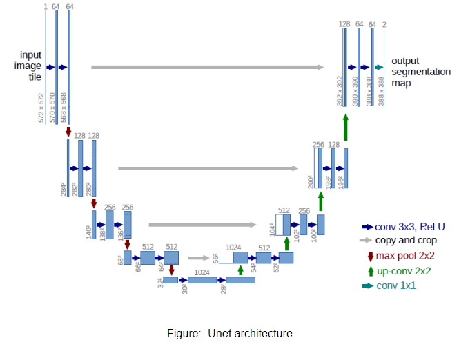
Mask-RCNN is an excellent deep learning model that can fulfill the tasks of detection, classification, and segmentation in very complicated environments. The problem is that the model’s good performance is based on the complexity and the ‘depth’ and ‘width’ of the model. The complexity of the model makes the parameters tuning part difficult, and the great depth and width of the model greatly increase the algorithm time. Unet is a model widely used in Biomedical Engineering for medical image analysis. It is an excellent model for medical image segmentation. Most of the medical images contain fewer objects than the images gathered in autonomous cars. As a result, unet doesn’t have the RPN and ROI Pooling layers. It first extracts feature maps from the original images, and then upsample the feature maps, concatenate the upsampled feature maps with the previous maps of the same size, when the upsampled feature map is of the same size as the input image, it is the output layer. Unet is similar to the mask branch of the Mask-RCNN model because the limited number of objects in medical images allows the unet to have a good performance in segmentation without the RPN and ROI pooling layers. In fact, unet can be regarded as a binary classification model, it classifies the pixels in the output layer into two categories based on whether the pixels belong to an object of a certain category. Figure below shows the unet architecture.
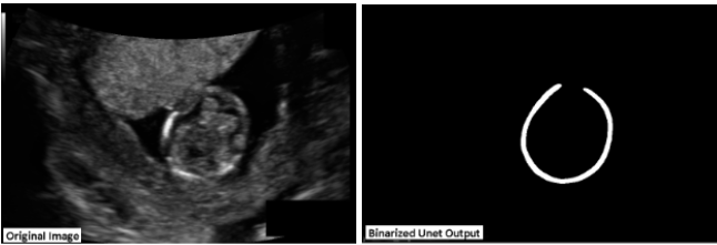
Two Figure shows two images from the project, Automated Measurement of Fetal Head Circumference, I finished last semester in ECE 5780 course (Computer Analysis of Biomedical Images). In the right image, the white pixels mean that these pixels belong to the fetal head circumference and the black ones not.
Unet Modifications
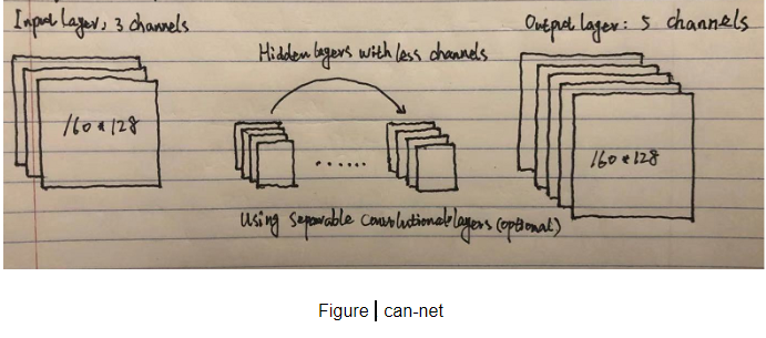
Similar to most medical images, the images in our project do not contain too many objects. With some simple modifications, we can obtain a new model that can be applied in our project. In this report, we will refer to our model as can-net
3 input channelsThe unet model was designed for segmenting the grayscale medical images, as a result, its input layer has only one channel. In our project, colors are quite useful information, we have three channels to represent the RGB color image. So the input layer of can-net has three channels.
5 output channels
Different from the fetal head circumference segmentation task, which segments objects of one category, our project segments objects of 5 different categories (ground, cola, beer, vehicle, head). One solution is that we can train 5 unet models and each is responsible for the segmentation of the objects of a certain category. The problem is that the processing time for 5 unet models is 5 times larger than a single unet model. In our project, the segmented images are highly related to each other. For example, in categories of ground, cola, beer, vehicle, different objects will never overlap with each other, for the vehicle and head, head will never be out of the vehicle because the head is part of the vehicle. Intuitively, the features extracted for the segmentation of one object can be helpful for the segmentation of the other objects. To reduce algorithm time, it’s better to have the 5 models share common feature maps extracted from the input images. For deep learning models, the front layers can be regarded as feature extraction layers and the end layers are responsible for their specified tasks. Based on our analysis, we can modify the output layer to let it have 5 channels, each channel is responsible for the segmentation of one category. Our tests showed that the can-net model with 5 output channels can precisely segment 5 objects with a little bit more time consuming than the model with one output channel.
Reduced widths of each layer
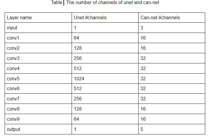
The unet model is designed as a general model applied in medical image analysis, not for a specified task. Every hidden layer of the unet has multiple channels. In our project, we will design a model for a certain application, the model doesn’t have to be so ‘wide’ to accommodate different input images. Most importantly, we will apply the model to the embedded system, which has limited computing resources but needs real-time processing speed. To reduce algorithm time, we can reduce the number of channels (width) of each layer. Table 1 shows a detailed comparison of the number of channels between unet and can-net.
Use separable convolutional layers (optional)
Separable convolutional layer is a substitute of normal convolutional layer in deep learning models. Figure below shows how a normal convolutional layer works. In this figure, the input map size is (64, 64, 3), the kernel size is (3, 3, 3), there are four kernels, after convolution (with padding), we obtained a map of shape (64, 64 ,4). The number of weights are 3*3*3*4 = 108.
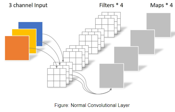
Figure below shows a corresponding separable convolutional layer of the above normal convolutional layer. In the separable convolutional layer, the first step is pointwise convolution. In this step, it uses three kernels of shape (3, 3, 1) to convolve the 3 input channels and obtains 3 output channels. The second step is depthwise convolution, it uses 4 kernels of shape (1, 1, 3) to convolve the 3 channels obtained in the first step, the result is a map of 4 channels. The number of weights are 3*3*3+4*3 = 39, nearly one third of the number of weights in the normal convolutional layer. Meanwhile, the two kinds of convolutional layers have input and output maps of the same sizes.
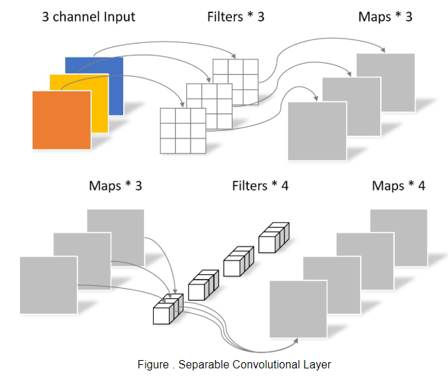
To generalize this, say, the input map has M channels and the output map has N channels. The normal convolutional layer has 3*3*M*N weights and the separable convolutional layer has 3*3*M+N*M weights. If both M and N are very large, the number of weights of the normal convolutional layer is nearly 9 times of that of the separable convolutional layer. Which means that the separable convolutional layer is much smaller in size than the normal convolutional layer. What’s more important for our project is that the separable convolutional layer can greatly reduce the training and inference time of the model. This is why separable convolutional layers are very popular in the models that are designed for the embedded systems, which have limited computing power. However, when we reduced the number of weights in the model, we also impaired the performance of it. In our tests we found that if we replaced all Conv2D layers with SeparableConv2D layers, there will be more errors in segmentation. So we didn’t use the separable convolutional layers in our project even if it can greatly reduce the algorithm time. One potential solution is replacing only some of the normal convolutional layers with the separable ones. If we have more time on the project, doing that is meaningful.
Image size
The size of the input images to can-net is 160*128. The images we obtained from the Pi camera is 320*240, in order to reduce the model inference time, we can resize the image to half of its original size, namely 160*120. But in can-net feature extraction layers, the feature map sizes have been downsampled 4 times, each time the feature map is half the size of the previous one. As a result, the width and height of the input images has to be multiples of 2^4 = 16. So we resize the input image to size of 160*128. Figure below is a picture illustrating how we modified the unet model and obtained our can-net model.
Traditional Computer Vision
Positioning
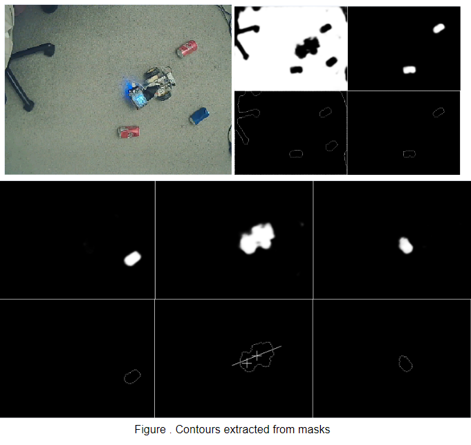
In order to control the vehicle to fulfill the tasks, we need to know exactly the positions of the vehicles and cans, and the direction of the vehicle. Given the masks, which are the segmented images of different objects, we can extract the contours of all objects. Chain code was used in this part. In the algorithm, we moved the pixel pointer along the horizontal lines from left to right, each time we encountered a point whose grayscale was larger than the threshold, we used the chain code method to compute the entire contour of that object. After that, we mark the contour on the mark image to avoid this object being searched again. To reduce the algorithm time, we searched the objects every four lines. Figure contours shows the mask of an image and the contours extracted from this mask.
We used the center points to denote the positions of the objects. The center points are the average value of the x and y coordinates of all contour pixels of an object.

To control the vehicle, we should know the direction of it. The direction of the vehicle can be denoted as a vector starting from the center of the vehicle and ending at the center of its head. The two points, the center of the vehicle and the center of the head are shown by two crosses in Figure contours

Where v is a vector denoting the direction of the vehicle and (chx, chy) is the center point of the head and (cvx, cvy) is the center point of the vehicle. But the center points of the vehicle and head are not precise enough. A more precise way of denoting the direction should be fitting a line using least squares method. The slope k and the intercept b on y axis can be computed by
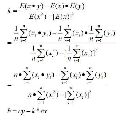
Where xi and yi are the coordinates of all pixels within the vehicle contour and cy and cy are the coordinates of the center point of the vehicle. Figure Center point shows the center points of the vehicle and its head and the fitting line of the vehicle.
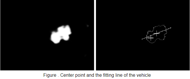
To make it easy for us to control the vehicle, we should use an angle in degree measurement to denote the direction of the vehicle. In other words, the angle denoting the direction of the vehicle should be in the range of [-180, 180). The angle beta can be computed by

But using this equation we will get an angle in the range of (-90, 90). Because the second parameter of atan2 is 1 > 0. It means that we will only get a line parallel to the vehicle direction, and the line may be in the opposite direction of the vehicle. The following equation helps solve this problem. Where chx is the x coordinate of the head and cvx is the x coordinate of the vehicle.

Vehicle Control
We should work out a route so that the vehicle can push the cans to the designated destinations. Figure Two routes shows two routes to push the can to the destination. There is no doubt that the red one is better. Because when the vehicle is pushing the can, an abrupt pilot (rotation) of the vehicle will lead to the can rolling away. So we should avoid abrupt rotation when the vehicle is pushing the can. The solution is, we first work out the rout from the can to the destination, namely, route B, then find the rotate point, a point that is a certain distance away from the can, and the vector from the can to the rotate point and the vector from the can to destination should be in opposite direction.
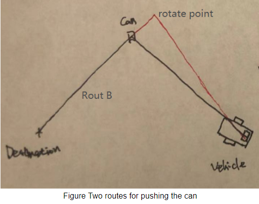
Figure Obstacles shows a more complicated situation. If we work out the route using the method described above, the vehicle will run into the obstacles.
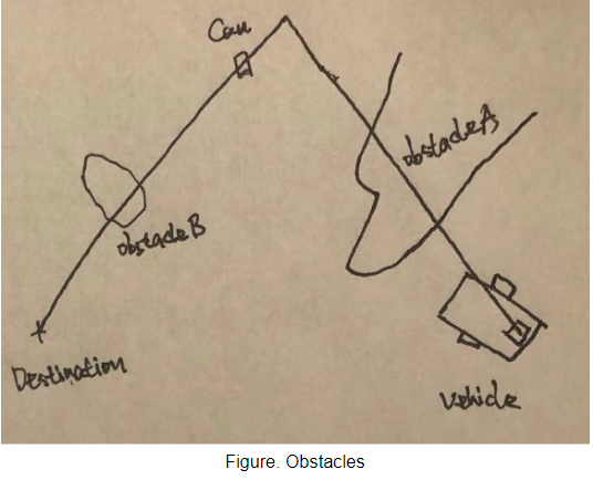
Figure Solution for obstacles shows the solution of this situation. First, expand the obstacles, shown in red. Second, get the contours of the expanded obstacles. Last, replace the line segments that overlap with the expanded obstacles with part of the contours of the obstacles. The red route ensures the vehicle will not run into the obstacles.
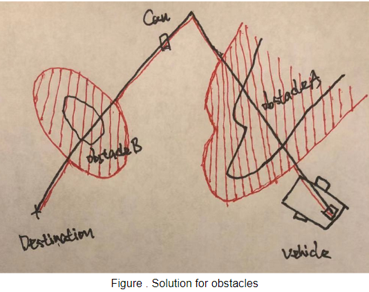
Figure example of the routeshows an example of the route for the vehicle (the read area) to circumvent the obstacle (the black area) to push the can (the green area) to the destination (the blue area).
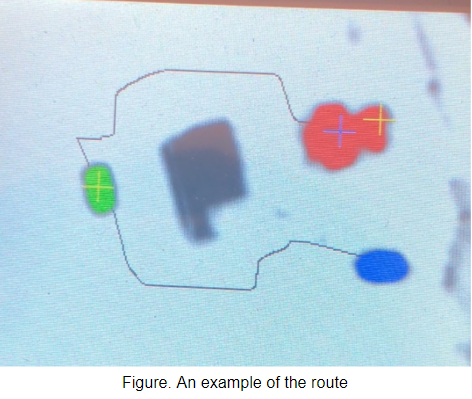
Even though we have the algorithm to compute the routes that ensure the vehicle does not run into the obstacles, we don’t show it in our final demo. Small camera view and variance in battery voltage often lead to the vehicle run into the obstacles. This will be explained in detail later.
Control algorithm
We control the vehicle based on the direction, angle and distance of the vehicle to the route. So we call our control algorithm direction-angle-distance control.
Direction
If the included angle of the direction of the vehicle and the direction of the route is larger than 45, we say the vehicle and the rout are in different directions. In this case, we rotate the vehicle. Figure .Different direction cases shows some examples of whether we should rotate the vehicle. (a)The included angle is larger than 45, direction of route - direction of vehicle > 0, the vehicle will rotate rightwards. (b)On the contrary, for this case, the vehicle will rotate leftwards. (d)The direction of the vehicle is perpendicular to the direction of the route, direction of route - direction of vehicle = 90 > 45, the vehicle will rotate rightwards. (d)In this case, the included angle of the direction of the vehicle and the direction of the route is less than 45, we don’t rotate the vehicle, we control the vehicle using angle-distance tuning method.
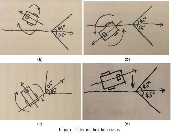
How to compute included angle
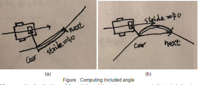
We have already talked about how to compute the direction of the vehicle. Now we will talk about how to compute the direction of the route and the included angles of the two directions. We use the two examples in figure below to illustrate this. In picture (a) we first find the point on the route that is nearest to the head of the vehicle, this point is referred to as the current point, move the current point 40 points forward along the route, we call this point the next point. The direction of the route can be denoted by the direction from the current point to the next point. If we use alpha to denote the direction of the route,
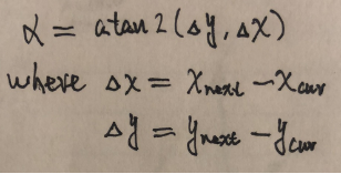
We used the same method to compute the direction of the route in (b) and find that the vehicle and the rout are parallel.
After computing the directions of the vehicle and the route, we can compute the included angle. We use theta to denote the included angle. Figure below is an example.
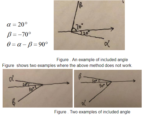
If we use the above method to compute the included angle, for the left and right images, respectively,

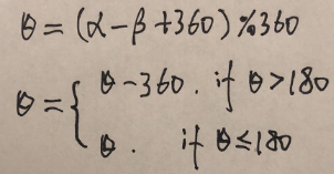
But in fact for the left image, theta = 50, because alpha is at the right of beta, for the right image, theta = -50, because alpha is at the left of beta. In fact, a method works for all cases is:
Angle-distance control
As we have discussed above, if the included angle of the vehicle is in the range of (-45, 45), we should use angle-distance control to control the vehicle. Angle-distance control is the control method that combines the included angle and the distance from the vehicle to the route, to work out a way to control the vehicle. First, for the angle part. In previous sections we already talked about methods to compute the included angle (theta) between the vehicle and the route. If theta > 0, it means the route is at the right side of the vehicle, turn the vehicle right by giving the left wheel a larger duty cycle and the right a smaller one and if theta smaller than 0, turn left. The difference of the duty cycles of the two wheels should be proportional to the absolute value of theta, which means that more correction for larger error and less correction for smaller error. Second, for the distance part. In fact, the distance should be a value larger than zero, it’s impossible that the distance from one object to another is less than zero. But in our project, in order to make the distance control method simple, we have positive and negative distances. A negative distance means the vehicle is at the left side of the route, and the positive means right. The absolute value of the distance from the vehicle to the route is the distance from the center point of the vehicle head to a nearest point on the route, which we have mentioned above. But, how can we know whether the head is at the left or right side of the route? Figure Four examples of distances shows four examples.
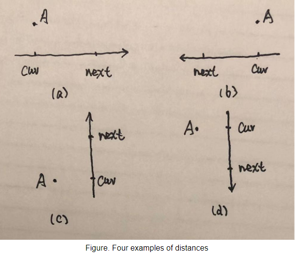
For figure Four examples of distances, both in (a) and (b), point A is above the route, the routes are in opposite directions, in (a) point A is at the left side of the route, in (b) point A is at the right side of the route. In (c), A is at the left of the route and in (d), A is at the right side of the route. In mathematics, the cross product or vector product of a and b is a vector that is perpendicular to both a and b, its direction is determined by the sign of the included angle from a to b. The sign of the vector product is the same as the sign of the angle theta (and sin(theta)), as figureThe vector product shows. So we can use the sign of the vector product of a and b, where a is the vector from the current point to A and b is the vector from the current point to the next point, to verdict whether A is at the left side of the route or right side.
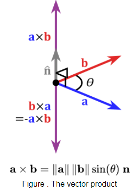
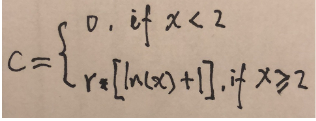
If we use (x0, y0) to denote vector a and (x1, y1) vector b. Then, the sign of a x b is the same as the sign of x0*y1-y0*x1. Until now, we can compute the signed distance from the center of the head to the route, and consequently we can use the signed distance to control the vehicle. If the head is at the left of the route, turn right, if the head is at the right of the route, turn left. In fact, the extent to which we turned the vehicle is not proportional to the distance from the head to the route. We used the following function to control the vehicle. It means that, if the absolute value of the distance is less than 2, we don’t turn the vehicle, if abs(distance) >= 2, the strength we turn the vehicle is r*(ln(x)+1). Where r is a magnification factor.
Why don't we use the strength proportional to the distance to turn the vehicle? In Figure below, the black line is the ln function, and the red line is our strength function.
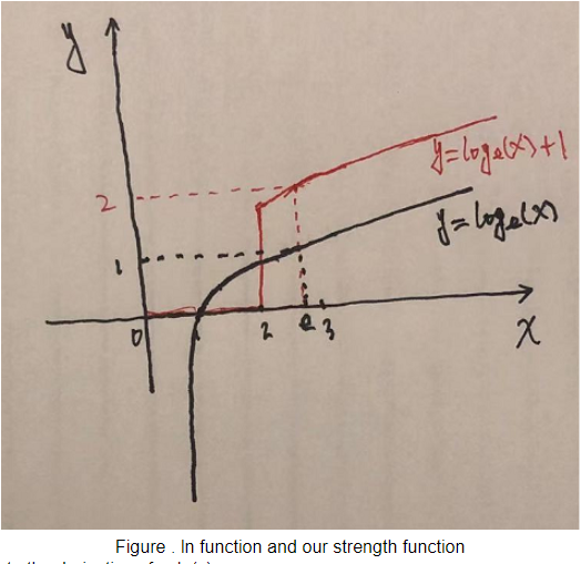
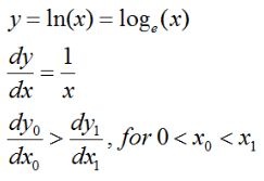
If we compute the derivative of y=ln(x). We can see that the derivative of y=ln(x), x>0, is monotonically decreasing, which means that larger values are less magnified than smaller ones. Why did we apply the ln function to the distance? Figure below shows two frequently observed cases in our project.
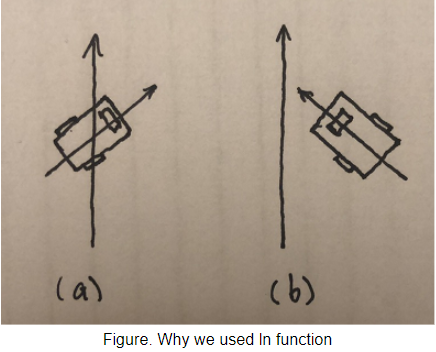
In (a), the head is not far away from the route, but the vehicle is running rightwards, we need to make the vehicle turn left. In (b) the head is far away from the route, but because the vehicle is moving leftwards, we don’t need to let the vehicle turn left. In other words, sometimes the vehicle is not far away from the route but it needs tuning, sometimes the vehicle is far away from the route but it doesn't need tuning. Finally, we sum up the strength generated by the included angle and the strength generated by distance, we will know how to control the vehicle. Combining the two methods results in a much better performance than only using one of them. In fact the two methods are complimentary in some cases. We can use example (b) in figure x to illustrate this. For this case, the head is at the right side of the route, the distance method will turn the vehicle left, but the angle method will turn the vehicle right because the included angle theta is larger than 0. As a result, the vehicle will not change its direction, this is the right way to avoid the vehicle being swinging along the route.
System Communication
Calling C functions in Python
In our project, a task is pushing one can to the destination. After finishing each task, we work out the route for the next task, this part of the algorithm was implemented in python. To fulfil the task, we should compute the position and direction of the vehicle for every frame image, this includes contours extraction and line fitting. If we use python to implement this, it will cost several seconds for processing one frame image (5 masks). If we used C++ to implement this, it would cost only about 0.01 seconds. So C is hundreds of times faster than python in some algorithms. So, here we will talk about how to implement algorithms using C++ and how to generate the .so file that can be called by python. In our project, we used C++ to extract contours, compute positions and fit lines from the 5 mask images. So, the input to the C++ function are 5 images, and output from the C++ function are several arrays, namely, contours and positions. In python code, we can use lists to represent the input images and output arrays. So, both the input and output of our C++ function are python lists. In C++ code, we first include the two files, ‘boost/python.hpp’ and ‘boost/python/numpy.hpp’. The two files enable us to use the data type ‘boost::python::list’, this is the python list in C++ code. Then the image data list can be transferred to C++ code via a parameter ‘boost::python::list& data’. To return the result to python, the return variable should also be the data in type ‘boost::python::list&’. Here we have a simple example illustrating how to build a C++ function whose inputs and outputs are python lists. Figure x shows a C++ code test5.cpp. The input to this function is a python list and an int variable, the output of this function is a list of all the values in the input list multiplied by the variable multi. In the Square function, data[i] is a python type data, we can use boost::python::extract
Testing
Model training
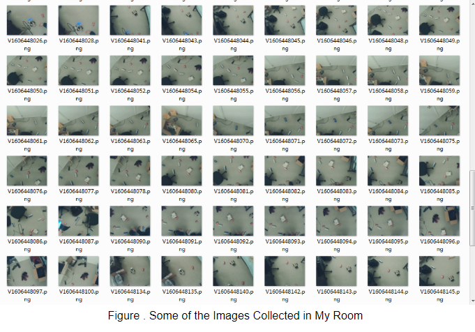
After designing our deep learning model, we will train it and use it to do the job of objects segmentation. To train the model, we collected the images of the vehicle, cans and obstacles on the floor, deleted some of the images that are not helpful, for example the ones that are quite similar to the previous images. Figure shows some of the images we collected in bedroom.
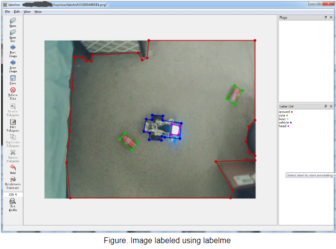
Then we used label me to label these objects. Figure x shows an example of the image labeled using labelme. In labelme, regions are denoted by polygons. After labeling each image, labelme will generate a .json file that includes the labeling information. We labeled a total of 201 images.
To feed the deep learning model, we will write a data generating function to generate the data, including images and masks, to be fed into the model. Opencv provides the function cv2.fillPoly that is useful here. FillPoly function can fill a polygon with a specified color given the sequenced coordinates of the polygon’s vertices, which are included in the json file. Data augmentation is a quite useful trick in deep learning to reduce overfitting, it can generate more data from the original given data. In our project, the images are top views of the ground, it’s meaningful to generate more images by horizontally and vertically flipping the original images. Figure below shows the images and masks generated by data augmentation, the top left image is the original image, the rest images are generated by flipping the original ones horizontally or vertically. The right images are the masks of the corresponding images on the left side. While training the model, we randomly feed the images or the generated ones with their masks into the model. For the masks, the white pixels represent ground, the black pixels represent obstacles and the colored pixels represent vehicle, cola cans, beer cans and vehicle screen (head), respectively.
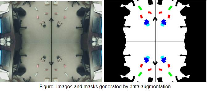
Figure below shows the input image and output masks of the trained can-net model, different objects are marked with different colors.
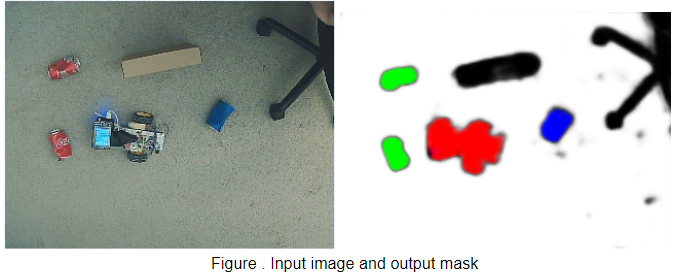
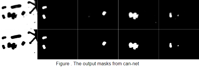
Figure output from can-net shows the output masks of different categories. The top 5 images are output masks from the can-net, the bottom 5 images are binarized images of the top 5 ones. For the top 5 images, the first is the segmented result of the ground, the second is the result of cola cans, the third the beer cans, the 4th the vehicle and the 5th the head. In the ground masks, the white pixels represent the ground, where the vehicle can run on, the black pixels are obstacles that the vehicle should circumvent. We can see that the box, chair feet and cans are recognized as obstacles. Note in the fifth image, the small white region is the wrong segmentation of can-net, our traditional algorithm will eliminate these regions.
Optimization on Algorithm Time
In our project, the camera Pi first analyzes the images gathered from the camera, and then sends commands to the vehicle Pi to control the vehicle. So, a fast algorithm is critical for our project. If the algorithm is slow, the vehicle may run into the obstacles before the camera can ‘see’ it. We have several approaches to optimize our program for a better performance.
Two processes reduce video delay time
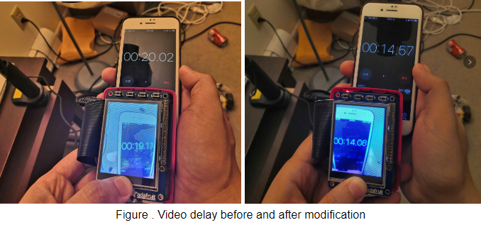
In our project, the time for processing each frame is about 0.25 seconds. But the video delay time is much larger than that. To measure the video delay, we used the camera to take the picture of my iphone, after processing the image using the algorithm, display the image on TFTPi. Then use another phone to take pictures of both the TFT Pi and my iPhone. From the pictures we can see the video delay time on the left image is 0.89 seconds, which is much larger than 0.25 seconds. The large difference between the video delay and the algorithm time is caused by the video buffer. In raspberry pi, there is a video buffer that stores the images that have not been read. The video flow of the raspberry pi is 30 fps (perhaps we can modify the fps but I didn’t find how to modify it), our algorithm time is 0.25s, the result is many frames will be stored in the video buffer, every time we read a frame from the buffer, we read the first one, namely the oldest one in the video buffer. To solve this problem, we created a new process that reads frames in buffers 40 times every second. Theoretically, in this way, the images it gathered from the image buffer is the newest one. The right image shows the video delay time has been reduced to 0.49 seconds after we modified our program.
A light deep learning model
We designed a deep learning model that can segment objects belonging to 5 categories rather than training 5 models each one responsible for the segmentation of one category, this helps save time. Moreover, we reduced the number of channels of each layer, which also helps accelerate the inference process. Finally, the inference time of our can-net model is about 0.20 seconds.
Implement some of the algorithms using C language
In our project, we should extract the contours of every object and the ground, and fit a line to denote the slope of the vehicle in every frame. Initially, I used python to do that job, only extracting contours costs several seconds. Later on I used C++ to implement these algorithms, the algorithm time has been reduced to 0.01 seconds, for this part, C++ algorithms are hundreds of times faster than python algorithms.
O3 optimization helps accelerate algorithms.
While compiling the C++ files, we can use -O3 option to get an optimized ‘.so’ file which is much faster than the one not optimized.
g++ -O3 alg_c.cpp -fPIC -shared -o alg_c.so -I/usr/include/python3.7 -I/usr/local/include/boost -L/usr/local/lib -lboost_python3
Our tests showed that our C++ algorithm is more than 10 times faster after -O3 optimization than before optimization.
Put images to different addresses helps make full use of the four CPU cores
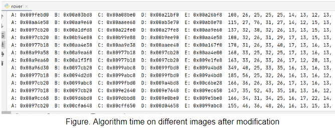
We used C++ to analyze the 5 masks (segmented images), each of which is of size (160,128) and one byte for a pixel. Initially in C++ code, I allocated a block of memory of size 160*128*5, and copied the 5 masks to the block. We used the same algorithm to process the 5 masks, but found that the algorithm time on the first image is much less than that on the other images. Figure x shows the algorithm time in cycles, marked by the red box. The total time for the 5 images are over 1 second.

Then we decided to split the 5 images to 5 separate files. So I allocated 5 blocks of memories each of which is of size 160*18, and put the 5 images to 5 blocks. That really helps. Figure x shows the time on 5 images after modification of my C++ program.
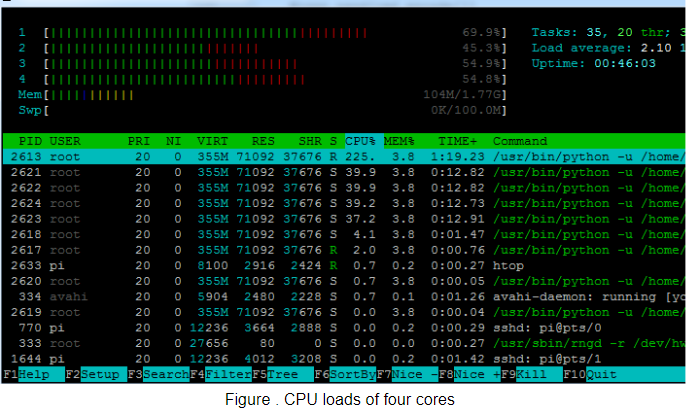
ecause the L1 and L2 caches are getting filed by the single large file. Each core on the ARM processor has an individual L1 data cache, if I put the 5 images to 5 blocks of memory that are not continuous, it could allow each image to become resident in L1 cache and allow for faster processing. We can use htop command to view the cpu loads of 4 cores, as figure x shows. There is not much difference among the cpu loads of four cores, I think this is because the deep learning model consumes much more computing resources. To compare the cpu loads of 4 cores on the C++ algorithm time, we can save the masks to the file system, then read these files and call the C++ function. But we didn’t spend time on that.
Opencv and numpy can help accelerate algorithms
Opencv and numpy have useful tools that can accelerate our algorithms. For example, the output masks from the deep learning model are of size (160,128), we should resize it to size (320,240) for further analysis. Bilinear interpolation is a good method. But it will be burdensome for us to fulfil the algorithm by coding. Opencv has the resize function, and it costs less time. In python, I also used np.hstack and np.vstack for the expansion of the objects, that really helps reduce algorithm time.
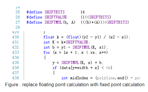
Use fixed point computation to replace floating point computation in C++
Generally speaking, floating point computation costs more time than fixed point computation, especially for the platforms that have no floating point accelerator. Figure below shows a method to replace floating point calculation with fixed point calculation. But when using this method, we should be careful of overflow.
Avoid using the functions that are time consuming
In our algorithm, when finding the nearest point on the route to the head, we can compute the distance from the points to the center head point, and find the smallest one. The distance between two points is sqrt((x1-x2)**2+(y1-y2)**2). In our code, we don’t need to use sqrt to compute the square root. We can find the minimum value of ((x1-x2)**2+(y1-y2)**2), and the square root of the minimum value is the distance between the head and the route. Sqrt is a time consuming function no matter in C++ or in python, use it less times can help reduce algorithm time.
Results & Conclusion
Comparison of our method with PID
PID control methods can be splitted into three methods, P, I, and D controls. P means tuning the system with the strength proportional to the error. Our distance control method is similar to this method except that our distance control applies a ln function to the error. D Control analysis the derivative of the error, the derivative means the ‘trend’ of the system. In fact, in our angle control, the included angle is the moving ‘trend’ of the vehicle, we are controlling the vehicle by analyzing the ‘trend’ of the movement of the vehicle. In fact, controlling the vehicle is more difficult than controlling some other systems. For example, if our vehicle is at the right side of the route running rightwards, we turn it left by a small angle, for the next step the vehicle is still running rightwards and away from the route because a little tuning does not change the running direction of the vehicle.
For the vision system, most of our expectations were successful completed as scheduled and planned. As we already discussed in the design and testing section, we will not address more in this result section.
vehicle circumventing obstacles
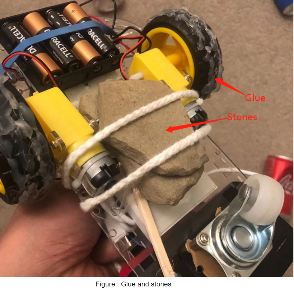
The view is small since our camera can only get images of size 320*240. We resize the images to size of (160*128) to accelerate the deep learning algorithm. If we hold our camera high, our camera can see the ground of a larger area, but the objects will be very small in pixels, it’s nearly impossible for a deep learning model (in fact, it is ‘shallow’ and ‘narrow’ and not deep, because we want to reduce algorithm time) to segment these small objects correctly. A solution to the small view is that we can use a camera of higher resolution. But larger images means more computing time. If we have more time working on this project, we can use the Movidius Neural Compute Stick to accelerate the deep learning inference time. It is said that this device can reduce the inference time of a large scale neural network to several milliseconds. We initially gathered images in my bedroom. We found that sometimes the vehicle will not move smoothly in my room because there is carpet on the floor. The small white wheel often got stuck on the carpet, especially when the battery's voltage is low. We then moved to my basement to do the experiment. The small white wheel will not get stuck on the cement ground of my basement. But the ground is very slippery. So our control method has a poor performance in the basement. We tried to solve this problem by adding glue to the wheel and fasten to stones at the bottom of the vehicle, as figure x shows, but not helpful. So we finally finished the project in my bedroom. It's a miserable experience every time we change our project because every time we should gather new images and label hundreds of pictures using labelme, that will cost us more that one day’s time.
Work out a real-time route
Currently, we use python to compute the route. Python is so slow so we only compute the route when the vehicle is not on the task. When the vehicle is on the task, and we move the object, the vehicle may not finish the task because it is still running according to the route computed before the task. It’s better to implement the route generating algorithm using C so that the Pi can work out the route after every frame. If we move the objects when the vehicle is moving, the vehicle can change its movements accordingly.
motor solution for torque
The torque of the motors are greatly affected by the voltage of the batteries. New batteries make the vehicle move and rotate very fast even given a low duty cycle, batteries having been used for more than one hour often make the vehicle stuck even give a high duty cycle. Sometimes the parameters of the control algorithm are not workable only because of the variance of battery voltage. It show as the figure below:
Future Work
What can be done to make the project better
We are very glad to have this opportunity to apply what we have learned from the computer vision course to the embedded system. But we only have a limited amount of time working on this project. The end of this semester seems so busy but interesting. We jotted down some ideas that may help make our project better given more time. Hope in the future, in our work or study time, we have the time and opportunity to test our ideas.
Error in segmentation
Sometimes there will be errors in segmentation. For example, some of the obstacles may be recognized as the vehicle. We can solve the problem by (1)Labeling more training data, currently we only have 201 images for training. (2)Using a deeper and wider neural network which can extract more useful features from the input images. (3) Using a deep learning model inference accelerator, such as Intel Movidius Neural Computing Stick, faster algorithms allows deeper models and better performance. (4)Using mask-rcnn model. This is an excellent model but needs more computing resources.
Use separable convolutional layers
We used separable convolutional layers, it can indeed save algorithm time but it also impairs the precision of the result. A potential solution is replacing some of the normal convolutional layers with separable convolutional layers.
Budget
| Vendor | Description | Quantity | Unit Cost($) | Total Cost($) |
|---|---|---|---|---|
| ECE Department | Raspberry Pi 3B | 1 | 35.00 | 70 |
| Amazon | Webcam | 1 | 20.00 | 20.00 |
| Total | 90 | |||
References
- separable convolutional layers
- How to build a function whose inputs and outputs are python lists.
- Mask-rcnn
- Unet
- Mean square error:
- Tensorflow
- Tflite:
- Vector product
- Log function
Work Distribution
For our can collector project, we work together closely. Yanda worked on motor control program and Jinling work on the vision system, but most of the work is done together in the Our basement and bedroom.
Code Appendix
alg_c.cpp
C++ implementation of the contour extraction, positioning and fitting algorithms.
can-net:
can-net model.
data.py
data generator.
end_model.py
can-net model.
end_train.py
Training program.
vehicle_receiver:
rover_receiver.py
The program running on vehicle Pi. It receives commands from the camera Pi and moves the
vehicle by one step.
rasp_vehicle
Code for camera Pi.
rover.py
Program for camera Pi.
rout.py
the algorithm for the route that we are currently using.
rout_bak.py
The algorithm for the route that can circumvent obstacles.